Exploratory Factor Analysis in R

Exploratory Factor Analysis (EFA) is a powerful statistical method used in data analysis for uncovering the underlying structure of a relatively large set of variables. It is particularly valuable in situations where the relationships between variables are not entirely known or when data analysts seek to identify underlying latent factors that explain observed patterns in data.

At its core, EFA helps in simplifying complex data sets by reducing a large number of variables into a smaller set of underlying factors, without significant loss of information. This technique is instrumental in various fields, including psychology, marketing, finance, and social sciences, where it aids in identifying patterns and relationships that are not immediately apparent.

The importance of EFA lies in its ability to provide insights into the underlying mechanisms or constructs that influence data. For example, in psychology, EFA can be used to identify underlying personality traits from a set of observed behaviors. In customer satisfaction surveys, it helps in pinpointing key factors that drive consumer perceptions and decisions.

Moreover, EFA is crucial for enhancing the validity and reliability of research findings. By identifying the underlying factor structure, it ensures that subsequent analyses, like regression or hypothesis testing, are based on relevant and concise data constructs. This not only streamlines the data analysis process but also contributes to more accurate and interpretable results.

In summary, Exploratory Factor Analysis is an essential tool in the data analyst’s arsenal, offering a pathway to decipher complex data sets and revealing the hidden structures that inform and guide practical decision-making. Its role in simplifying data and uncovering latent variables makes it a cornerstone technique in the realm of data analysis and interpretation.

What is exploratory factor analysis in R?

Introduction to Exploratory Factor Analysis (EFA)

Now, let’s understand what is EFA in detail. Exploratory Factor Analysis (EFA) is a statistical technique used to uncover the underlying structure of a relatively large set of variables. It’s often employed when researchers or data analysts do not have a preconceived notion about how variables are grouped together. The primary goal of EFA is to identify the number of latent variables (factors) that can explain the patterns of correlations among observed variables.

When to Use EFA

EFA is particularly useful in the early stages of research when you have a dataset with multiple variables and are interested in discovering how they relate to each other. It helps in reducing the dimensionality of the data by identifying the most important factors, which can simplify further analysis and interpretation. Now we have understood what is EFA in detail.

Key Concepts in EFA

• Latent Variables (Factors): Unobserved variables that are inferred from the observed data.
• Factor Loadings: Correlations between observed variables and factors. They indicate how much a factor explains a variable.
• Communalities: The proportion of each variable’s variance that can be explained by the factors.
• Eigenvalues: Measure the amount of variance in the observed variables explained by each factor. Factors with eigenvalues greater than 1 are typically considered significant. Now we have understood what is EFA in detail.

Basic Concept and Mathematical Foundation

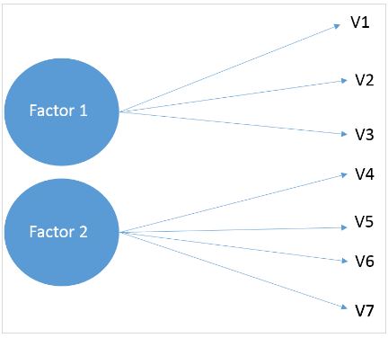
• The fundamental idea behind EFA is that there are latent factors that cannot be directly measured but are represented by the observed variables.
• Mathematically, EFA models the observed variables as linear combinations of potential factors plus error terms. This model is represented as: X = LF + E, where X is the matrix of observed variables, L is the matrix of loadings (which shows the relationship between variables and factors), F is the matrix of factors, and E is the error term.
• Factor loadings, which are part of the output of EFA, indicate the degree to which each variable is associated with each factor. High loadings suggest that the variable has a strong association with the factor.
• The process involves extracting factors from the data and then rotating them to achieve a more interpretable structure. Common rotation methods include Varimax and Oblimin.

Differences from Confirmatory Factor Analysis (CFA)

• EFA differs from Confirmatory Factor Analysis (CFA) in its purpose and application. While EFA is exploratory in nature, used when the structure of the data is unknown, CFA is confirmatory, used to test hypotheses or theories about the structure of the data.
• In EFA, the number and nature of the factors are not predefined; the analysis reveals them. In contrast, CFA requires a predefined hypothesis about the number of factors and the pattern of loadings based on theory or previous studies.
• EFA is more flexible and is often used in the initial stages of research to explore the possible underlying structures. CFA, on the other hand, is used for model testing and validation, where a specific model or theory about the data structure is being tested against the observed data.

Exploratory Factor Analysis is a powerful tool for identifying the underlying dimensions in a set of data, particularly when the relationships between variables are not well understood. It serves as a foundational step in many statistical analyses, paving the way for more detailed and hypothesis-driven techniques like Confirmatory Factor Analysis. Now we have understood what is EFA in detail.

Here is an overview of efa in R and what is EFA in detail. We will also learn some factor analysis example.

As the name suggests, EFA is exploratory in nature – we don’t really know the latent variables, and the steps are repeated until we arrive at a lower number of factors. In this tutorial, we’ll look at EFA using R. Now, let’s first get the basic idea of the dataset. We will also learn some factor analysis example.

1. The Data

This dataset contains 90 responses for 14 different variables that customers consider while purchasing a car. The survey questions were framed using a 5-point Likert scale with 1 being very low and 5 being very high. The variables were the following:

• Price
• Safety
• Exterior looks
• Space and comfort
• Technology
• After-sales service
• Resale value
• Fuel type
• Fuel efficiency
• Color
• Maintenance
• Test drive
• Product reviews
• Testimonials

Download the coded dataset now.

2. Importing WebData

Now we’ll read the dataset present in CSV format into R and store it as a variable. We will also learn some factor analysis example.

[code language=”r”] data <- read.csv(file.choose(),header=TRUE) [/code]

It’ll open a window to choose the CSV file and the `header` option will make sure that the first row of the file is considered as the header. Enter the following to see the first several rows of the data frame and confirm that the data has been stored correctly.

[code language=”r”] head(data) [/code]

3. Package Installation

Now we’ll install the required packages to carry out further analysis. These packages are `psych` and `GPArotation`. In the code given below, we are calling `install.packages()` for installation.

[code language=”r”] install.packages(‘psych’) install.packages(‘GPArotation’) [/code]

4. Number of Factors

Next, we’ll find out the number of factors that we’ll be selecting for factor analysis statistics. This is evaluated via methods such as `Parallel Analysis` and `eigenvalue`, etc. We will also learn some factor analysis example.

Parallel Analysis

We’ll be using the `Psych` package’s `fa.parallel` function to execute the parallel analysis. Here we specify the data frame and factor method (`minres` in our case). Run the following to find an acceptable number of factors and generate the `scree plot`:

[code language=”r”] parallel <- fa.parallel(data, fm = ‘minres’, fa = ‘fa’) [/code]

The console would show the maximum number of factors we can consider. Here is how it’d look.

“Parallel analysis suggests that the number of factors = 5 and the number of components = NA“

Given below in the `scree plot` generated from the above code:

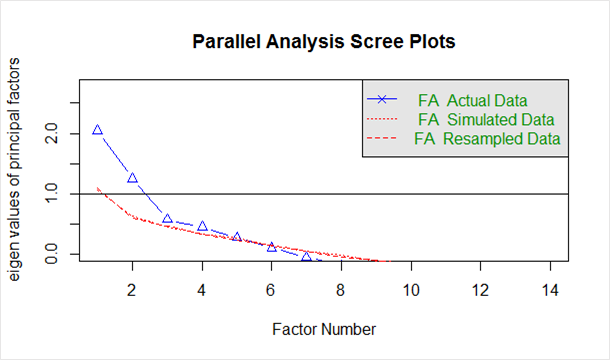
The blue line shows eigenvalues of actual data and the two red lines (placed on top of each other) show simulated and resampled data. Here we look at the large drops in the actual data and spot the point where it levels off to the right. Also, we locate the point of inflection – the point where the gap between simulated data and actual data tends to be minimum.

Looking at this plot and parallel analysis, anywhere between 2 to 5 factors would be a good choice.

Factor Analysis

Now that we’ve arrived at a probable number of factors, let’s start off with 3 as the number of factors. In order to perform factor analysis, we’ll use the `psych` packages`fa()function. Given below are the arguments we’ll supply:

• r – Raw data or correlation or covariance matrix
• nfactors – Number of factors to extract
• rotate – Although there are various types of rotations, `Varimax` and `Oblimin` are the most popular
• fm – One of the factor extraction techniques like `Minimum Residual (OLS)`, `Maximum Liklihood`, `Principal Axis` etc.

In this case, we will select oblique rotation (rotate = “oblimin”) as we believe that there is a correlation in the factors. Note that Varimax rotation is used under the assumption that the factors are completely uncorrelated. We will use `Ordinary Least Squared/Minres` factoring (fm = “minres”), as it is known to provide results similar to `Maximum Likelihood` without assuming a multivariate normal distribution and derives solutions through iterative eigendecomposition like a principal axis.

Run the following to start the analysis.

[code language=”r”] threefactor <- fa(data,nfactors = 3,rotate = “oblimin”,fm=”minres”) print(threefactor) [/code]

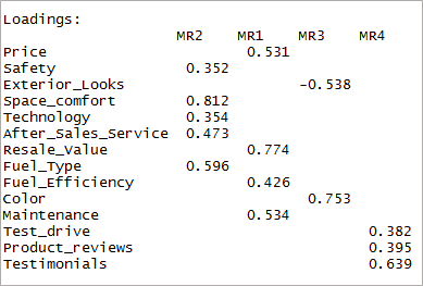
Here is the output showing factors and loadings:

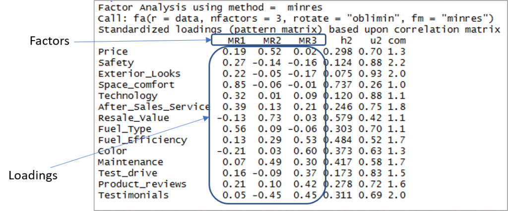
Now we need to consider the loadings of more than 0.3 and not loading on more than one factor. Note that negative values are acceptable here. So let’s first establish the cut-off to improve visibility.

[code language=”r”] print(threefactor$loadings,cutoff = 0.3) [/code]

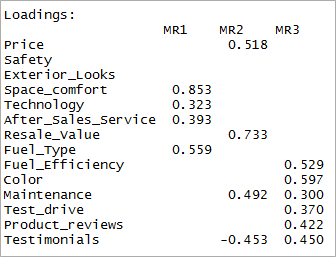
As you can see two variables have become insignificant and two others have double-loading. Next, we’ll consider the ‘4’ factors.

[code language=”r”] fourfactor <- fa(data,nfactors = 4,rotate = “oblimin”,fm=”minres”) print(fourfactor$loadings,cutoff = 0.3) [/code]

We can see that it results in only single-loading. This is known as the simple structure.

Hit the following to look at the factor mapping.

[code language=”r”] fa.diagram(fourfactor) [/code]

Adequacy Test

Now that we’ve achieved a simple structure it’s time for us to validate our model. Let’s look at the factor analysis output to proceed.

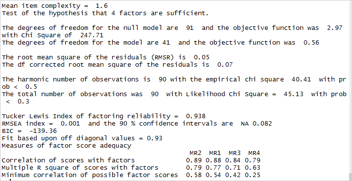
The root means the square of residuals (RMSR) is 0.05. This is acceptable as this value should be closer to 0. Next, we should check the RMSEA (root mean square error of approximation) index. Its value, 0.001 shows a good model fit as it is below 0.05. Finally, the Tucker-Lewis Index (TLI) is 0.93 – an acceptable value considering it’s over 0.9.

Naming the Factors

After establishing the adequacy of the factors, it’s time for us to name the factors. This is the theoretical side of the analysis where we form the factors depending on the variable loadings. In this case, here is how the factors can be created.

The Importance of EFA in Data Analysis

Exploratory Factor Analysis (EFA) is a critical tool in data analysis, highly valued for its ability to simplify complex datasets, reduce dimensions, and reveal latent variables. The significance of EFA in various industries and research fields is multifaceted:

Simplifying Data

• EFA helps in making large sets of variables more manageable. By identifying clusters or groups of variables that are closely related, EFA reduces the complexity of data. This simplification is crucial in making the data more understandable and in facilitating clearer, more concise interpretations.

Reducing Dimensions

• In datasets with numerous variables, EFA serves as an efficient method for dimensionality reduction. It consolidates information into a smaller number of factors, making it easier to analyze without a significant loss of original information. This reduction is particularly useful in fields like machine learning and statistics, where handling large numbers of variables can be computationally intensive and challenging.

Uncovering Latent Variables

• One of the most significant advantages of EFA is its ability to identify latent variables. These are underlying factors that are not directly observed but inferred from the relationships between observed variables. In psychology, for example, EFA can reveal underlying personality traits from observed behaviors. In marketing research, it can identify consumer preferences and attitudes that are not directly expressed.

Role in Various Industries and Research Fields

• Market Research: In market research, EFA is used to understand consumer behavior, segment markets, and identify key factors that influence purchase decisions.
• Psychology and Social Sciences: EFA is extensively used in psychological testing to identify underlying constructs in personality, intelligence, and attitude measurement.
• Healthcare: In the healthcare sector, EFA helps in understanding the factors that affect patient outcomes and in developing scales for assessing patient experiences or symptoms.
• Finance: EFA assists in risk assessment, portfolio management, and identifying underlying factors that influence market trends.
• Education: In educational research, EFA is utilized to develop and validate testing instruments and to understand educational outcomes.

In each of these fields, EFA not only aids in data reduction and simplification but also provides critical insights that might not be apparent from the raw data alone. By revealing hidden patterns and relationships, EFA plays a pivotal role in informing decision-making processes, developing strategic initiatives, and advancing scientific understanding. The versatility and applicability of EFA across different domains underscore its importance as a fundamental tool in data analysis.

Conclusion

In this tutorial for analysis in r, we discussed the basic idea of EFA in R (exploratory factor analysis in R), covered parallel analysis, and scree plot interpretation. Then we moved to factor analysis in R to achieve a simple structure and validate the same to ensure the model’s adequacy. Finally arrived at the names of factors from the variables. Now go ahead, try it out, and post your findings in the comment section.

If you’re intrigued by the possibilities of EFA and other data analysis techniques, we invite you to delve deeper into the world of advanced data solutions with PromptCloud. At PromptCloud, we understand the power of data and the importance of extracting meaningful insights from it. Our suite of data analysis tools and services is designed to cater to diverse needs, from web scraping and data extraction to advanced analytics.

Whether you’re looking to harness the potential of big data for your business, seeking to understand complex data sets, or aiming to transform raw data into strategic insights, PromptCloud has the expertise and tools to help you achieve your goals. Our commitment to delivering top-notch data solutions ensures that you can make data-driven decisions with confidence and precision.

Explore our offerings, learn more about how we can assist you in navigating the ever-evolving data landscape, and take the first step towards unlocking the full potential of your data with PromptCloud. Visit our website, reach out to our team of experts, and join us on this journey of data exploration and innovation.

---

 

Frequently Asked Questions (FAQs)

What is the factor analysis function in R?

Factor analysis in R is a statistical method used to describe variability among observed, correlated variables in terms of potentially lower unobserved variables, called factors. Essentially, it helps in understanding the underlying structure of a data set.

What is PCA factor analysis in R?

Principal Component Analysis (PCA) in R is a technique used for dimensionality reduction, simplifying the complexity in high-dimensional data while retaining trends and patterns. PCA transforms the original variables into a new set of variables, the principal components, which are orthogonal (as uncorrelated as possible), and which account for as much of the variability in the data as possible.

What is the difference between EFA and CFA?

The main difference between Exploratory Factor Analysis (EFA in R) and Confirmatory Factor Analysis (CFA) lies in their objectives and methods:

• Exploratory Factor Analysis (EFA) is used when the relationships among variables are not known. EFA explores the data to find patterns and identify underlying factors. It’s a ‘discovery’ tool used to understand data structure without predefined notions.

• Confirmatory Factor Analysis (CFA), on the other hand, is used to test hypotheses or theories about the relationships among variables. In CFA, the researcher has a specific idea about how many factors there are and which variables are linked to which factors. It’s a ‘testing’ tool used to confirm or reject preconceived notions about data structure.

EFA is about exploring and discovering patterns in data, while CFA is about testing specific hypotheses regarding these patterns

How do you interpret exploratory factor analysis results?

How does one interpret the rotated factor loadings in practical terms?

Interpreting rotated factor loadings involves understanding the relationship between the variables and the underlying factors they are associated with. A higher loading of a variable on a specific factor indicates a stronger relationship with that factor. In practical terms, researchers should look for variables that load significantly on the same factor and group them together to represent a latent construct or dimension of the data being analyzed. This process involves qualitative judgment to name and interpret these factors based on the variables that load highly on them, considering the theoretical framework and the context of the study.

What are the best practices for handling missing data when performing EFA?

Handling missing data in exploratory factor analysis requires careful consideration to avoid biasing the results. One common approach is to use listwise or pairwise deletion, where observations with missing values are excluded from the analysis. However, this can lead to a significant reduction in sample size and potential loss of valuable information. A more sophisticated method is to impute missing values using techniques such as mean imputation, regression imputation, or multiple imputation. These methods fill in missing values based on the information available in the dataset, allowing for a more complete and accurate factor analysis. The choice of method depends on the nature of the missing data and the assumptions underlying each imputation technique.

How can one validate the results obtained from EFA? 

Validating the results obtained from exploratory factor analysis involves several strategies to ensure the stability and generalizability of the factor structure. One common approach is to split the sample into two halves and perform EFA separately on each half to see if similar factor structures emerge. Another method is to conduct a confirmatory factor analysis (CFA) on a new sample to test whether the factor structure identified through EFA holds. Additionally, researchers might use goodness-of-fit indices in CFA to assess how well the model fits the data. These validation techniques help confirm the reliability of the factor solution and its applicability across different samples or contexts.

What is meant by factor analysis?

Factor analysis is a statistical method used to describe variability among observed, correlated variables in terms of a potentially lower number of unobserved variables called factors. Essentially, it aims to identify underlying relationships between variables to reduce the dimensionality of data. This technique is useful in various fields, including psychology, finance, and social sciences, to identify latent constructs that cannot be measured directly but can be inferred from the observed variables.

The process involves:

1. Identifying the underlying factors: Factor analysis explores large datasets to find hidden patterns, suggesting that multiple variables are actually related to a smaller number of factors. These factors represent underlying processes or constructs that influence the observed variables.
2. Reducing dimensionality: By identifying these factors, factor analysis reduces the number of variables to consider. For example, instead of dealing with dozens of individual variables, you might find that they are predominantly influenced by a few underlying factors.
3. Data summarization and simplification: This reduction allows for a more manageable, simplified interpretation of complex data sets, facilitating data analysis and interpretation.

There are mainly two types of factor analysis:

• Exploratory Factor Analysis (EFA): Used when the underlying structure among the variables is unknown. EFA is a technique to explore the data to find any patterns or relationships between variables.
• Confirmatory Factor Analysis (CFA): Used when researchers have a specific hypothesis or theory about the structure in the data. CFA tests whether the data fit the hypothesized measurement model.

The results of factor analysis are used to enhance our understanding of data by revealing the underlying structure, aiding in the development of theories, improving measurement instruments, and contributing to more efficient data reduction and variable selection strategies.

What is the goal of the factor analysis?

The goal of factor analysis is to identify the underlying relationships among a set of observed variables and to represent this information in a simpler form. This statistical technique aims to achieve several key objectives:

1. Dimensionality Reduction: Factor analysis reduces the complexity of data by identifying a smaller number of factors that can explain the correlations among a larger set of observed variables. This makes the data more manageable and interpretable.
2. Identifying Underlying Constructs: It seeks to uncover latent variables (factors) that are not directly observed but inferred from the observed variables. These underlying constructs can explain patterns in the data and how variables are related.
3. Data Simplification: By reducing the number of variables to a smaller set of factors, factor analysis simplifies data analysis, making it easier to visualize and understand complex data sets.
4. Improving Measurement Instruments: In research and psychometrics, factor analysis helps in the development and refinement of measurement instruments (such as surveys and tests) by identifying the most relevant items that measure underlying constructs.
5. Theoretical Development and Testing: The technique aids in the development and testing of theories by revealing the structure of relationships among variables, thus providing empirical evidence to support theoretical constructs.
6. Data Compression: Factor analysis allows for data compression, enabling large datasets to be represented more compactly without losing significant information, which is particularly useful for further statistical analysis or machine learning applications.

Ultimately, the goal of factor analysis is to provide a deeper understanding of the data by identifying its underlying structure, facilitating more effective data interpretation, and supporting decision-making processes based on simplified, yet comprehensive insights into the relationships between variables.

What are the steps of factor analysis?

Factor analysis is a systematic method used to explore and understand the underlying structure of a set of variables. The process typically involves several key steps:

Define the Problem and Select Variables

• Identify the specific objectives of the factor analysis and select the variables to be included in the analysis. This step requires a clear understanding of the research questions and the nature of the data.

Check Suitability of Data

• Assess the appropriateness of your data for factor analysis. This includes checking for sufficient correlations among variables (since factor analysis is based on identifying these correlations). Tools like the Kaiser-Meyer-Olkin (KMO) measure of sampling adequacy and Bartlett’s test of sphericity can help determine if your data is suitable.

Choose the Extraction Method

• Decide on a method to extract the factors. The most common approach is Principal Component Analysis (PCA), used for initial explorations of the data. Another approach is Principal Axis Factoring (PAF), which is more suitable for identifying underlying theoretical constructs.

Determine the Number of Factors

• Decide how many factors to retain. This decision can be guided by criteria such as eigenvalues greater than 1 (Kaiser Criterion), the scree plot, and the percentage of variance explained by factors. The goal is to retain factors that meaningfully contribute to understanding the data structure.

Rotate the Factors

• Apply rotation methods to make the interpretation of factors easier. Rotation can be orthogonal (e.g., Varimax, which assumes factors are uncorrelated) or oblique (e.g., Direct Oblimin, allowing for correlations among factors). Rotation helps clarify the relationship between factors and variables.

Interpret the Factors

• Analyze the rotated factor loadings (correlations between variables and factors) to interpret the factors. Factors are usually interpreted by examining which variables load strongly on them, providing insight into the underlying constructs represented by each factor.

Compute Factor Scores

• (Optional) Calculate factor scores for each observation if you wish to use the identified factors for further analysis. Factor scores can be used as variables in subsequent analyses, such as regression.

Validate the Model

• Assess the adequacy and validity of the factor analysis model, possibly using techniques like confirmatory factor analysis (CFA) in a separate sample to confirm that the identified structure fits the data well.

Report the Results

• Clearly document and report the methodology, results, and interpretations of the factor analysis, including the rationale for key decisions made during the process.

These steps provide a structured approach to uncovering the latent structure within a set of variables, helping researchers and analysts make informed decisions based on the insights gained through factor analysis.

What is the exploratory factor analysis used for?

Exploratory Factor Analysis (EFA) is used for several key purposes in both research and applied settings, primarily focusing on uncovering the underlying structure of a dataset without imposing any prior assumptions about the nature or number of factors that influence the observed variables. Its main uses include:

Identifying Underlying Constructs

EFA helps in discovering latent variables or factors that cannot be directly measured but influence the observed variables. This is particularly useful in psychological, sociological, and educational research, where constructs like intelligence, satisfaction, or socio-economic status need to be inferred from multiple measured variables.

Reducing Dimensionality

By identifying a smaller number of factors that account for the majority of the variance in a large set of variables, EFA reduces the complexity of the data. This simplification makes it easier to understand the data and facilitates further analysis by focusing on the most significant underlying dimensions.

Improving Measurement Instruments

EFA is often used in the development and refinement of questionnaires and tests. By determining which items cluster together on the same factors, researchers can improve the reliability and validity of these instruments, ensuring that they effectively measure the intended constructs.

Theory Development and Testing

In the early stages of research, EFA can be instrumental in theory development by revealing patterns and relationships among variables that were not previously apparent. It can provide empirical support for theoretical constructs and generate hypotheses for further study.

Data Preprocessing

Before applying more complex statistical analyses or machine learning algorithms, EFA can be used as a preprocessing step to identify the most relevant variables and eliminate redundancy. This can enhance the performance and interpretability of subsequent analyses.

Identifying New Patterns and Relationships

EFA can uncover new, unexpected patterns and relationships between variables that can lead to novel insights and discoveries. This is particularly valuable in fields where the data are complex and multifaceted, such as genomics, behavior science, and market research.

In summary, exploratory factor analysis is a versatile tool used to explore data structures, reduce dimensionality, improve measurement accuracy, and facilitate theory development. Its utility spans various disciplines, making it a fundamental technique in the toolbox of researchers and analysts.

What is exploratory factor analysis APA?

When referring to “Exploratory Factor Analysis (EFA) APA” within the context of research and academic writing, it usually pertains to the guidelines and standards set by the American Psychological Association (APA) for reporting the results of an EFA. The APA is widely recognized for its publication manual, which provides comprehensive guidelines for the formatting and structuring of academic papers in the social and behavioral sciences, including how to report statistical analyses like EFA.

Here are some key points to consider when reporting EFA results in accordance with APA guidelines:

Description of the Method

• Clearly describe the EFA procedure, including the rationale for using EFA, the extraction method (e.g., Principal Axis Factoring, Maximum Likelihood), and the rotation method used (e.g., Varimax, Direct Oblimin), if applicable.

Assessment of Suitability

• Report on the assessment of data suitability for factor analysis. This includes mentioning tests and criteria used, such as the Kaiser-Meyer-Olkin (KMO) measure of sampling adequacy and Bartlett’s test of sphericity.

Factor Selection

• Explain the criteria for determining the number of factors to retain, such as eigenvalues greater than 1, scree plot examination, and the total variance explained by the factors.

Factor Loadings

• Present the factor loadings (correlations between variables and factors) in a table format. According to APA style, tables should be clear and include captions explaining what they represent. It’s common to highlight or only report loadings above a certain threshold (e.g., greater than .30 or .40) for clarity.

Factor Interpretation

• Discuss how the factors were interpreted based on the loadings. This involves naming the factors and describing the theoretical constructs they are believed to represent.

Rotation

• If rotation is used, specify the type of rotation and justify its use. Also, discuss how rotation affected the interpretation of the factors.

Factor Scores

• If factor scores are computed and used in subsequent analyses, describe how they were calculated and utilized.

Reliability Analysis

• Often, researchers report the reliability of the items loading on each factor (e.g., Cronbach’s alpha) to assess the internal consistency of the items associated with each factor.

When writing up EFA results, adhering to APA guidelines ensures that the report is clear, professional, and provides sufficient detail for readers to understand the analysis and its implications fully. The APA Publication Manual offers comprehensive instructions on presenting statistical analyses and results, making it an essential resource for researchers in psychology and related fields.

Sharing is caring!